Using layouts

Table of contents

• Introduction
• Layout definition
• Classes of layouts
  • Discrete and continuous layouts
  • Synchronicity of layouts
  • How animation affects synchronicity
• Choice of graph
  • The problem of large graphs
  • Metrics for subgraph selection
• Choice of layout
  • Builtin layouts versus external extensions
  • Default layout
  • Geometric layouts
  • Hierarchical layouts
  • Force-directed layouts
• Advanced layout use cases
  • Interactive use of layouts
  • Headless use of layouts
  • Batching and layouts
• Conclusion

Introduction

One of the first things to decide when visualising a graph is how lay out the nodes on the screen. A good layout can give a comprehensive view of the data. The choice of which particular layout to use is key, but equally important is the choice of how and when to use a layout.

Cytoscape supports several layouts, and it supports using layouts in several ways. This tutorial gives an overview of how to use layouts generally and when each layout is useful specifically.

Layout definition

A layout is simply a mapping function: It maps a node to a position. A layout takes as input a set of nodes and edges along with a set of options.

The set of nodes of edges, or collection, passed to a layout indicates which graph elements should be considered in the layout. Each node that is passed to a layout is positioned by the layout. Passed edges provide the layout with topology that can help to determine where nodes should be placed. For example, many layouts will organise nodes such that each node is in close proximity to its neighbourhood. Because a layout takes a set of elements as input, a layout can be used on the entire graph or on a subgraph (cy.layout() versus eles.layout()).

The set of options differs from layout to layout. These options allow you to configure how the layout runs by tuning the layout algorithm’s parameters. For example, many layouts have options to control how close nodes are to one another. Other common options allow for setting the resultant node positions using animation. By tweaking the layout options for your dataset, you can often get a better visual result than by using the defaults.

Classes of layouts

Discrete and continuous layouts

There are two main classes of layout, discrete and continuous.

A discrete layout sets node positions all at once. The nodes go immediately from their previous positions to their resultant layout positions; this makes this class of layout relatively cheap to run. The nodes are generally organised in a geometric pattern.

A continuous layout sets node positions over several iterations, typically through a force-directed algorithm. Each iteration sets a new node position. This creates a natural animation effect, though the underlying layout algorithm might or might not create a smooth transition between iterations. While a continuous layout is generally more expensive to run as compared to a discrete layout, a continuous layout may give more sophisticated results.

Synchronicity of layouts

There is a major distinction between these classes of layouts with respect to synchronicity.

A discrete layout is synchronous: The resultant positions are synchronously set such that you can access those resultant node positions on the line of code following layout.run().

A continuous layout is asynchronous: It runs iterations over time, without monopolising the main thread. You can not read resultant layout positions for a continuous layout on the line following layout.run(). Instead, you must use events or promises to run code after the layoutstop event.

How animation affects synchronicity

Animation options can alter the properties of continuous and discrete layouts. If a discrete layout is run as an animation via animate: true, then that layout is no longer synchronous. Further, a continuous layout may be configured to disable animation via animate: false. This makes the layout run all its iterations at once, albeit still asynchronously. This can make a continuous layout give its end result quicker. A continuous layout may also support animate: 'end', which animates in a similar manner to a discrete layout: The nodes are animated directly from the start positions to the end positions — avoiding potentially unaesthetic middle iteration positions.

Choice of graph

The first step in choosing a layout is choosing the graph or subgraph on which the layout is run. This is an important consideration. It is often a mistake to simply put an entire large dataset in the graph and run a layout on the entire graph. Consider what questions might be answered for a user with the data, and select subgraphs that can help to answer those questions.

The problem of large graphs

The root issue with large graphs is that it is difficult for a person to visually parse so many data points at once. Even assuming that you never have performance issues with large graphs and that you make an ideal choice of layout, large graphs usually just become visual noise. Choice of layout can help with that issue to some degree. Large, highly-connected graphs tend to be more or less a hairball regardless of choice of layout.

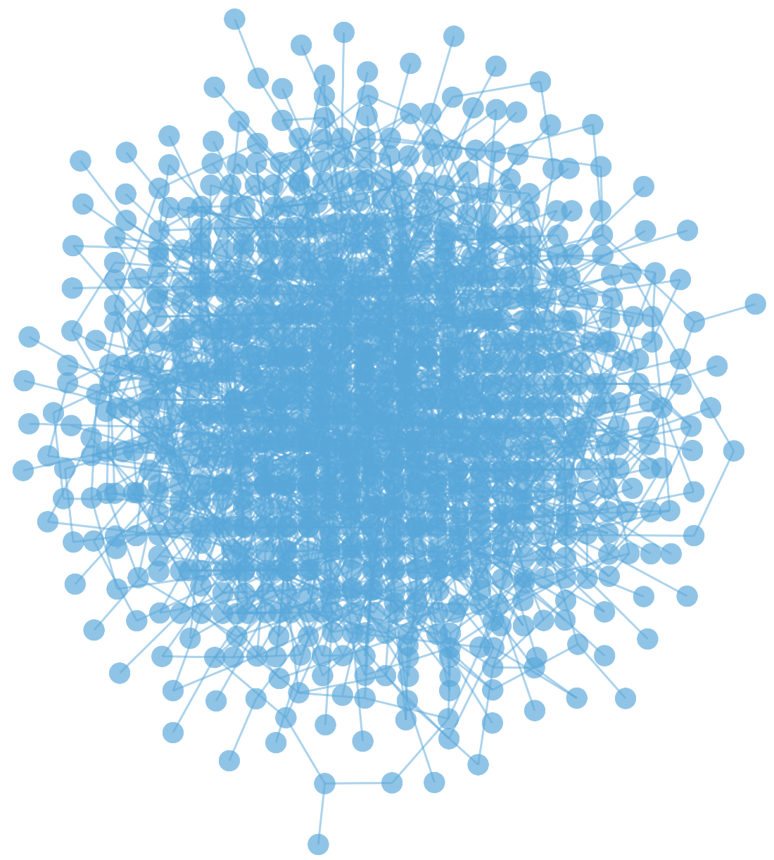
The problem, then, is to filter the elements to show only a relevant subset of the graph that a user could easily parse — and to allow the user easy navigation from one chosen subset to another one. You may load in subgraphs dynamically from your database, such as Neo4j or Neptune, if your dataset is very large. Alternatively, you may simply show and hide subgraphs using the Cytoscape API, if your dataset is small enough to load into a single Cytoscape instance.

Metrics for subgraph selection

A subgraph can be selected for display and layout based on metrics.

One useful metric is topology combined with score: You can select a subgraph based on the graph topology relative to a chosen locus (e.g. N hops away from a chosen node), using some score or ordinal ranking to cut down that topological set to a reasonable size. When you have a ranking within a subset, you can also use a pagination-like approach to flip through to lower-scoring elements in the topological subset (e.g. using a slider or stepper).

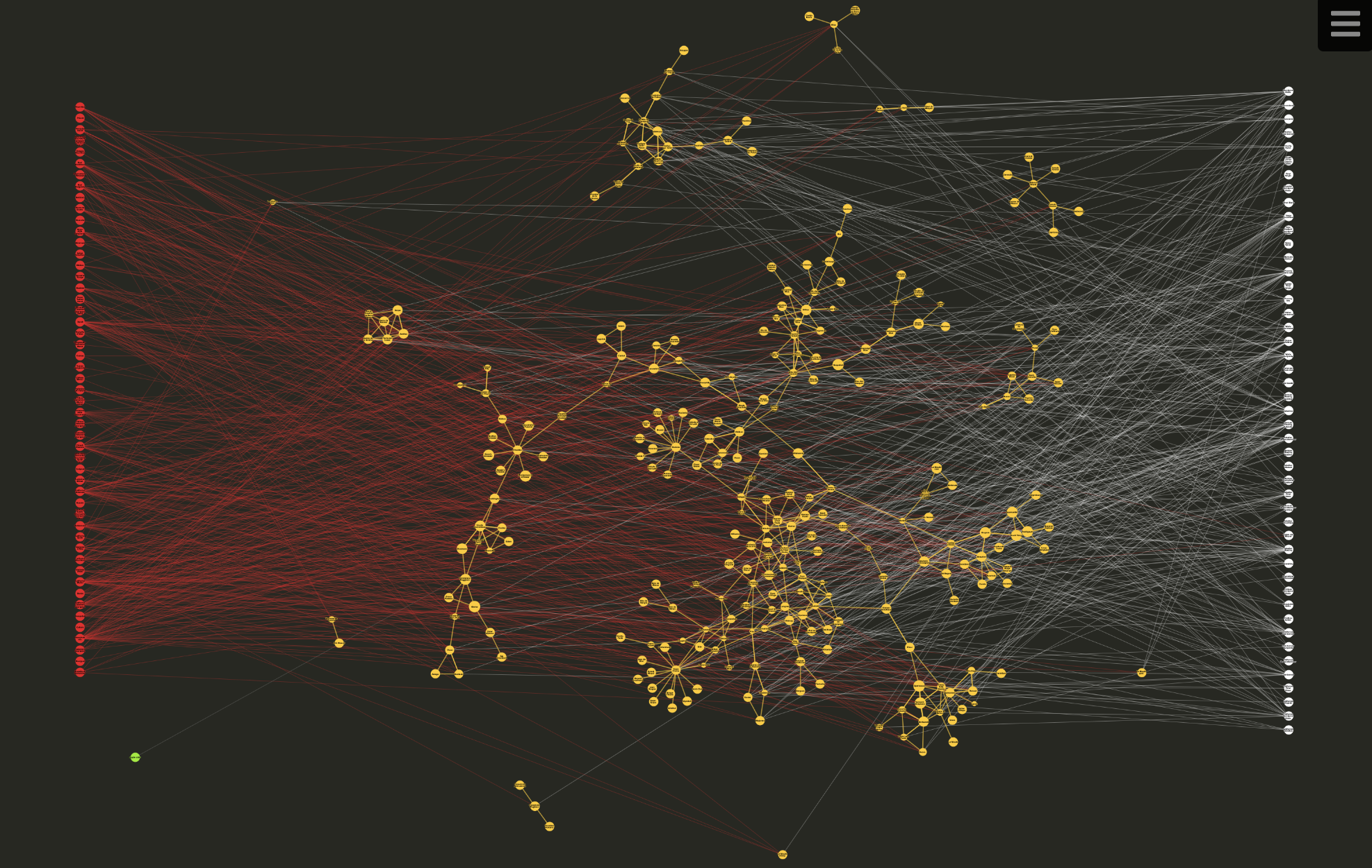
A simple example of a topological approach is the Wine & Cheese Map: The red and white wine edges are normally hard to see, like a hairball. By using filtering and layout based on the clicked node, the red and white edges of interest are more easily seen.

Serverside graph databases, such as Neo4j and Neptune, have algorithms that can be used to find relevant subgraphs. For example, centrality is a typical metric used to indicate relative importance of nodes within a graph. These metrics can be used to query the server for a relevant subgraph that is sent to the client and loaded into a Cytoscape visualisation.

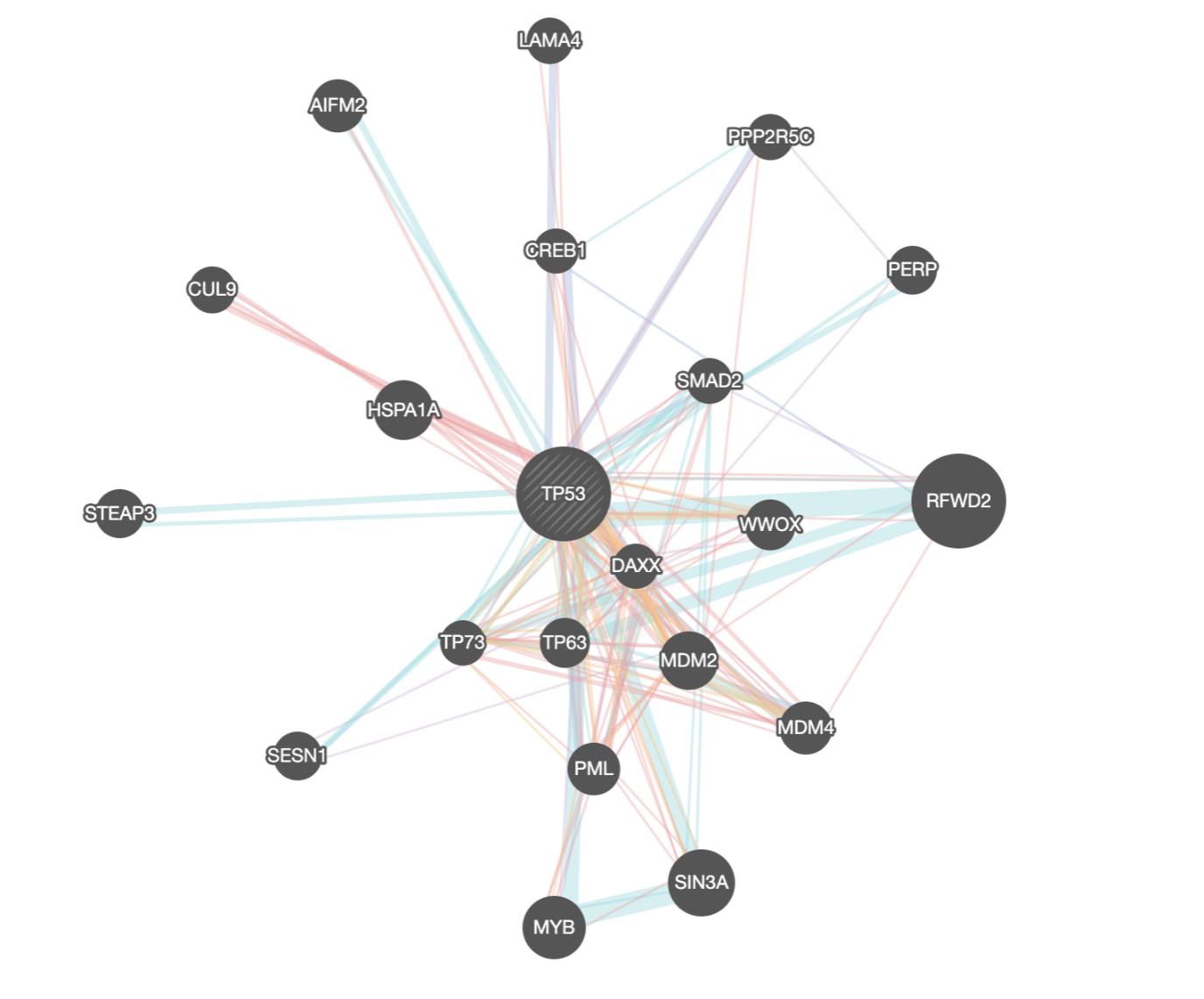
An example of this algorithmic subgraph approach is GeneMANIA, an app from the University of Toronto that shows relationships between genes in various model organisms. Just as it would be a mistake in other apps, it would be a mistake in GeneMANIA to present all the data to the user at once. The human genome contains on the order of 20,000 genes. You could try to plop all that data into a single graph visualisation. It would not be comprehensible, and further most users are probably only interested in particular subsets of the data. (Consider Google as an example: Do most users want to see all of Google’s webpage-webpage graph at once, or are users interested in particular, relevant subsets?)

So then, GeneMANIA has a serverside algorithm that allows the user to query for a set of genes of interest (e.g. TP53). The result is the subgraph of genes and interactions most related to the query genes. The analytics for GeneMANIA have shown over the years that the vast majority of users are interested in only a single query gene, which reinforces the importance of using relevant subgraphs.

Choice of layout

Once you have decided on an appropriate graph to use, your next task is to select a particular layout.

Builtin layouts versus external extensions

All layouts in Cytoscape.js are extensions. A number of layout extensions are included in the default cytoscape package for convenience. The builtin layouts are commonly used and they are small in file size. Other layouts, which are large or less frequently used, are left as external extensions. These external extensions can be easily integrated into your app by importing them and calling cytoscape.use(someLayoutExtension).

Default layout

If no layout is specified at initialisation of a Cytoscape graph, the grid layout is applied. The grid layout is an inexpensive layout that easily shows all nodes in the graph, so it is a natural default: It allows you to visually verify that the graph has correctly loaded.

You might not specify the graph elements at initialisation, instead opting to add the elements via cy.add(). When using this method, nodes are initially positioned at the points specified in the postition of each node’s JSON representation. If you do not have defined positions, then the nodes will be placed at the origin (0, 0) by default. You may run a layout following your call to cy.add() in order to set positions to the added nodes.

Preset layout

The preset layout is typically used at initialisation when you want to place the nodes at predetermined positions. Those positions are specified in each node’s position field in its JSON representation. Alternatively, the positions may be specified functionally via the positions layout option. You must use the preset layout for this usecase at initialisation, otherwise the predefined positions are overridden by the default grid layout.

Geometric layouts

These layouts organise the graph into common geometric shapes:

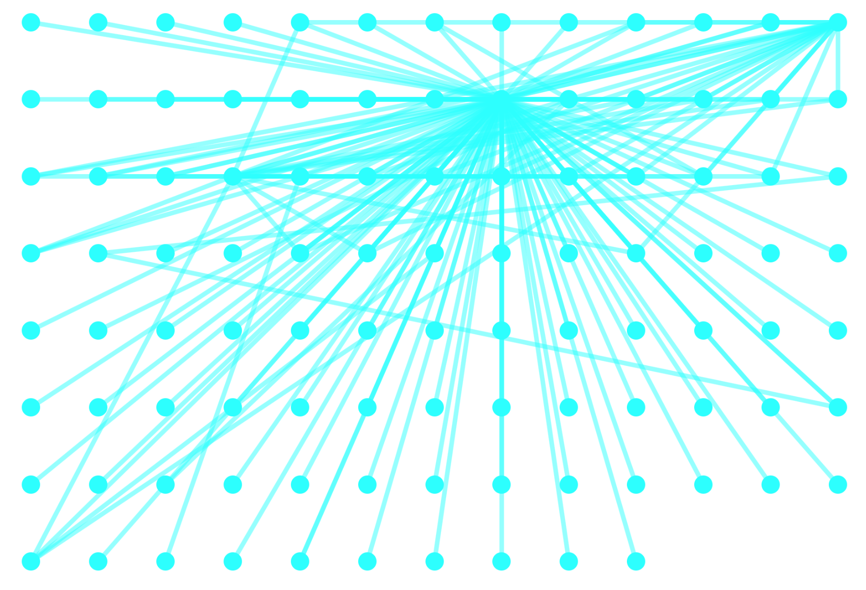
grid : The grid layout organises the nodes in a well-spaced grid. The nodes are placed from left to right and top to bottom, in the order they are passed to the layout. You can control the order by calling eles.sort().layout() or by ordering the elements as they are added to the graph. By default, the nodes are placed in a grid that fits the available viewport space well. If you can think of your nodes as being organised into several columns with one class of node per column — or similarly for rows — then the grid layout is a good fit. You can customise exactly which nodes go in which rows or columns. 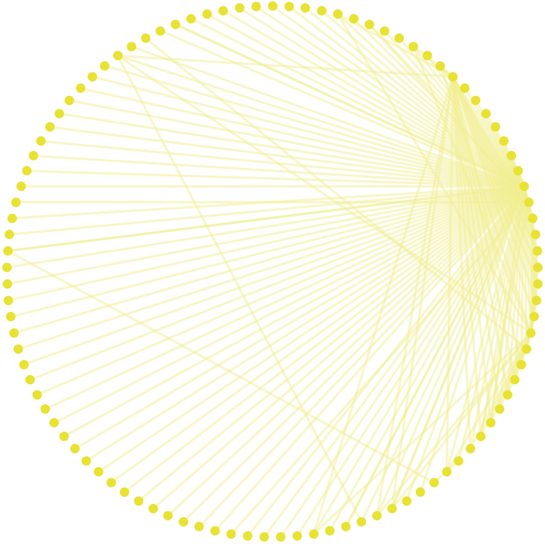For example, a bipartite layout is just a two-column case of a grid layout.

circle : The circle layout organises the nodes into a circle. By default, the nodes are placed clockwise from the 12 o’clock position, in the order that they are passed to the layout. You can control the order of the nodes by calling eles.sort().layout() or by ordering the elements as they are added to the graph. This layout helps to highlight the density of edges connected to different nodes, especially when the edges are made semitransparent.

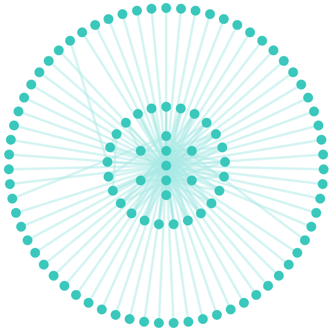
concentric : The concentric layout organises the nodes into concentric circles, based on the specified metric. The nodes with the highest metric values are placed in the innermost circle, and the metric values of the nodes descend for each outward circle. Each circle has nodes with metric values between a specified range, with the nodes within a circle sorted accordingly. This layout is useful for highlighting relative importance of the nodes, and its visual effect can be reinforced by creating a style mapper to the metric — e.g. nodes with larger metric values are darker in colour.

avsdf : The avsdf layout is another circle layout. Whereas the circle layout is useful when you want to order the nodes yourself, the avsdf layout is useful when you want to automatically order the nodes to try to avoid edge overlap.

Hierarchical layouts

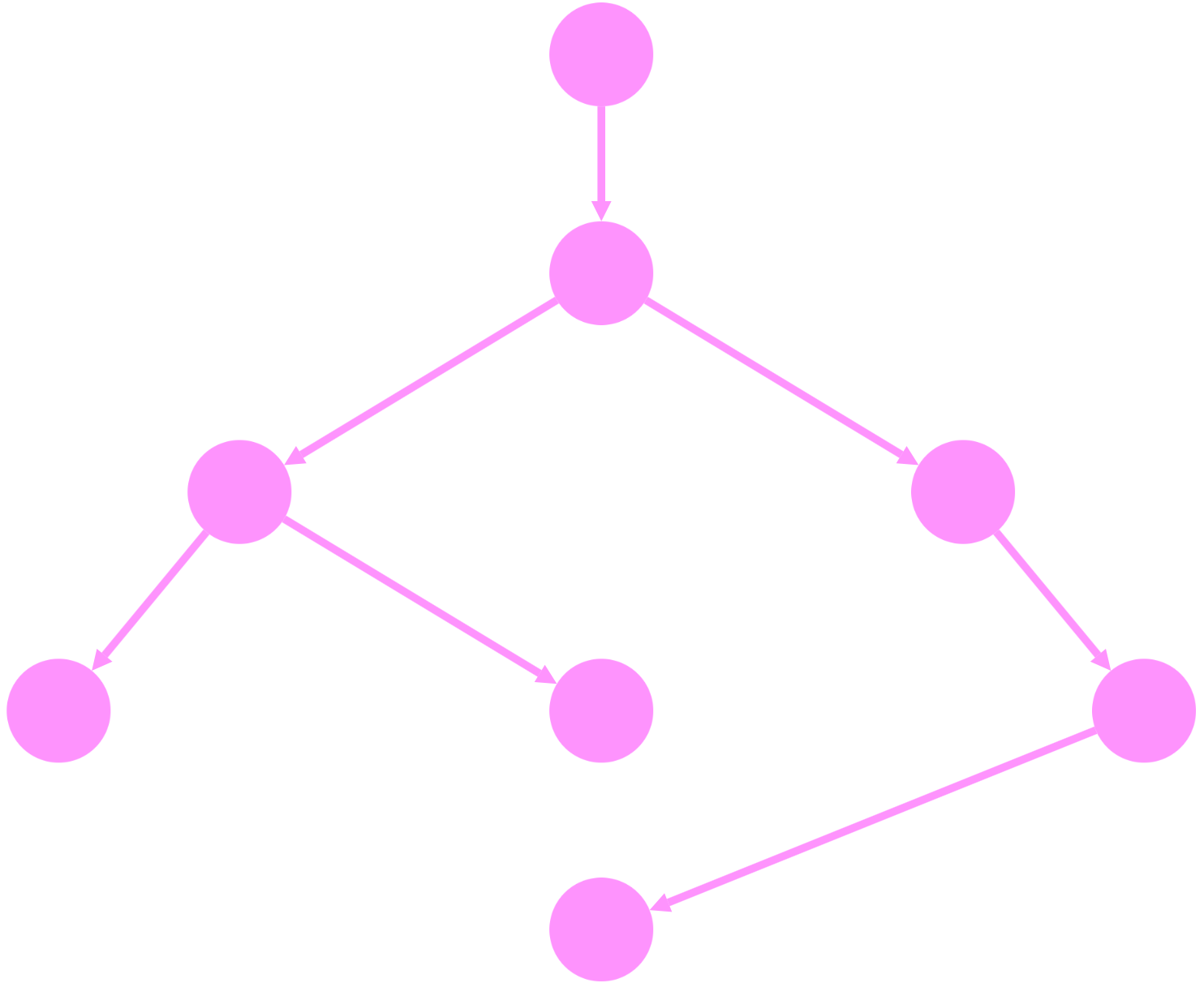
Hierarchical layouts work well for trees and directed acyclic graphs (DAGs). If your graph is directed — predecessor-successor relationships, such as in a binary search tree — and without cycles, then a hierarchical layout is a good fit. Traditional hierarchical layouts often pair well with taxi-styled edges.

Most hierarchical layouts are fairly similar, but they differ in important ways:

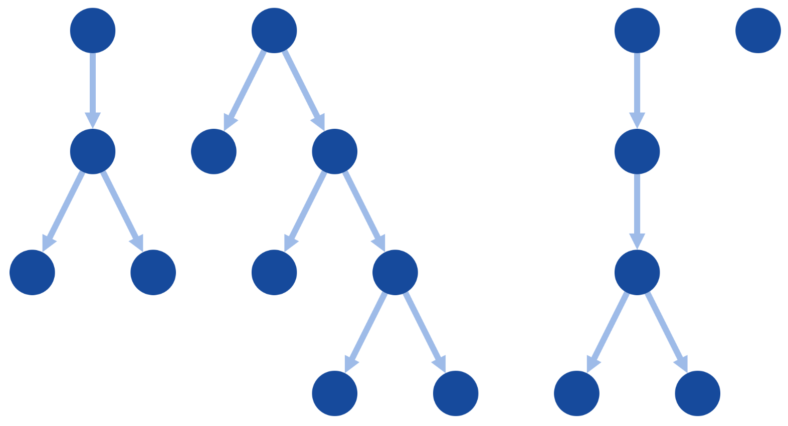
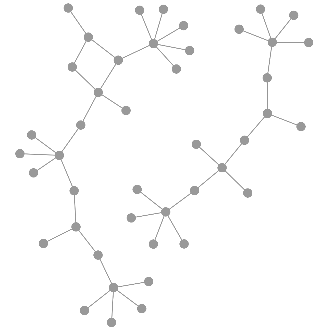
dagre : The dagre layout is a traditional hierarchical layout. It looks like how people typically draw binary trees on a whiteboard: It has a nice inverted V shape from one level to the next. This should be one of the first layouts that you try if your graph is a DAG.

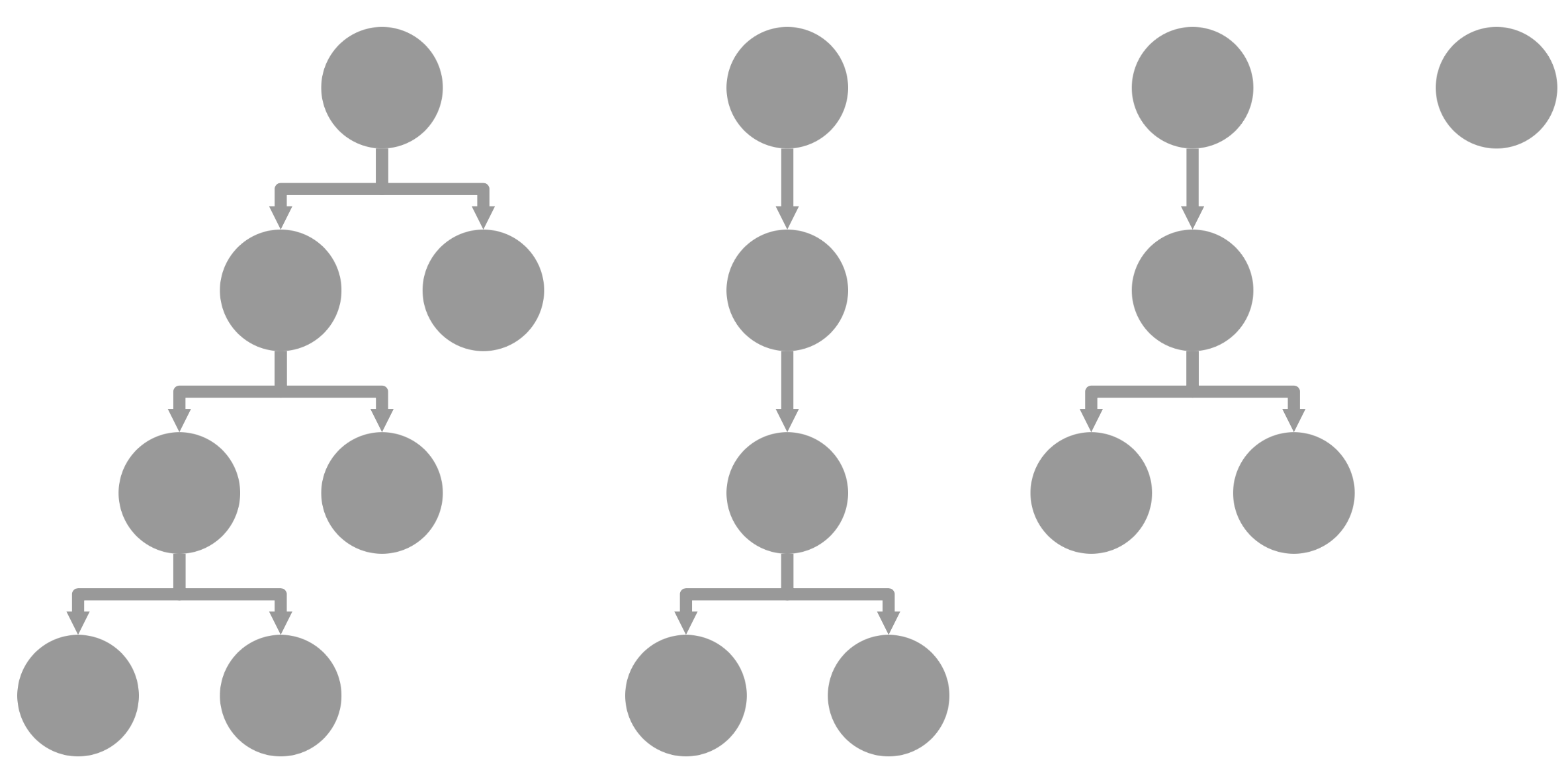
breadthfirst : The breadthfirst layout organises the nodes in levels, according to the levels generated by running a breadth-first search on the graph. This layout gives a less traditional result for DAGs than other layouts, but it uses space more efficiently.

concentric : The concentric layout can be made hierarchical by using the breadth-first search level as the metric. Though this results in a space-efficient result, it is less traditional than a typical top-down hierarchical layout.

elk : The elk layout contains several different layout algorithms. The layered and mrtree algorithms are traditional hierarchical layouts. For many trees, the results of elk probably will not differ much from dagre, and dagre has a smaller file size. The results of elk may differ from dagre to a greater degree for complex DAGs. Compare the results of both layouts and see which suits your dataset best.

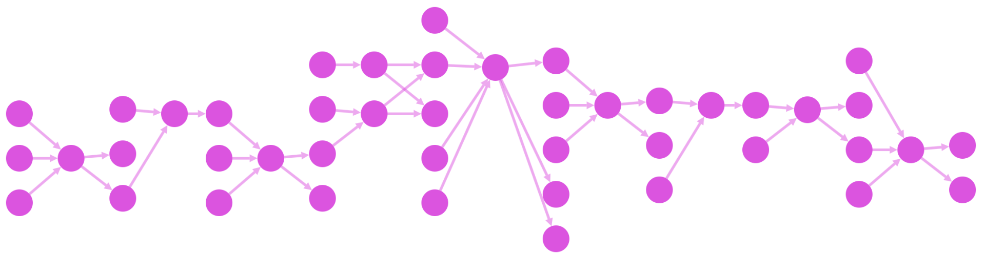
klay : The klay layout is a traditional hierarchical layout. It is the predecessor to the layered algorithm in elk. You may want to use klay for its smaller file size, if the layered algorithm of elk does not differ significantly for your dataset.

Force-directed layouts

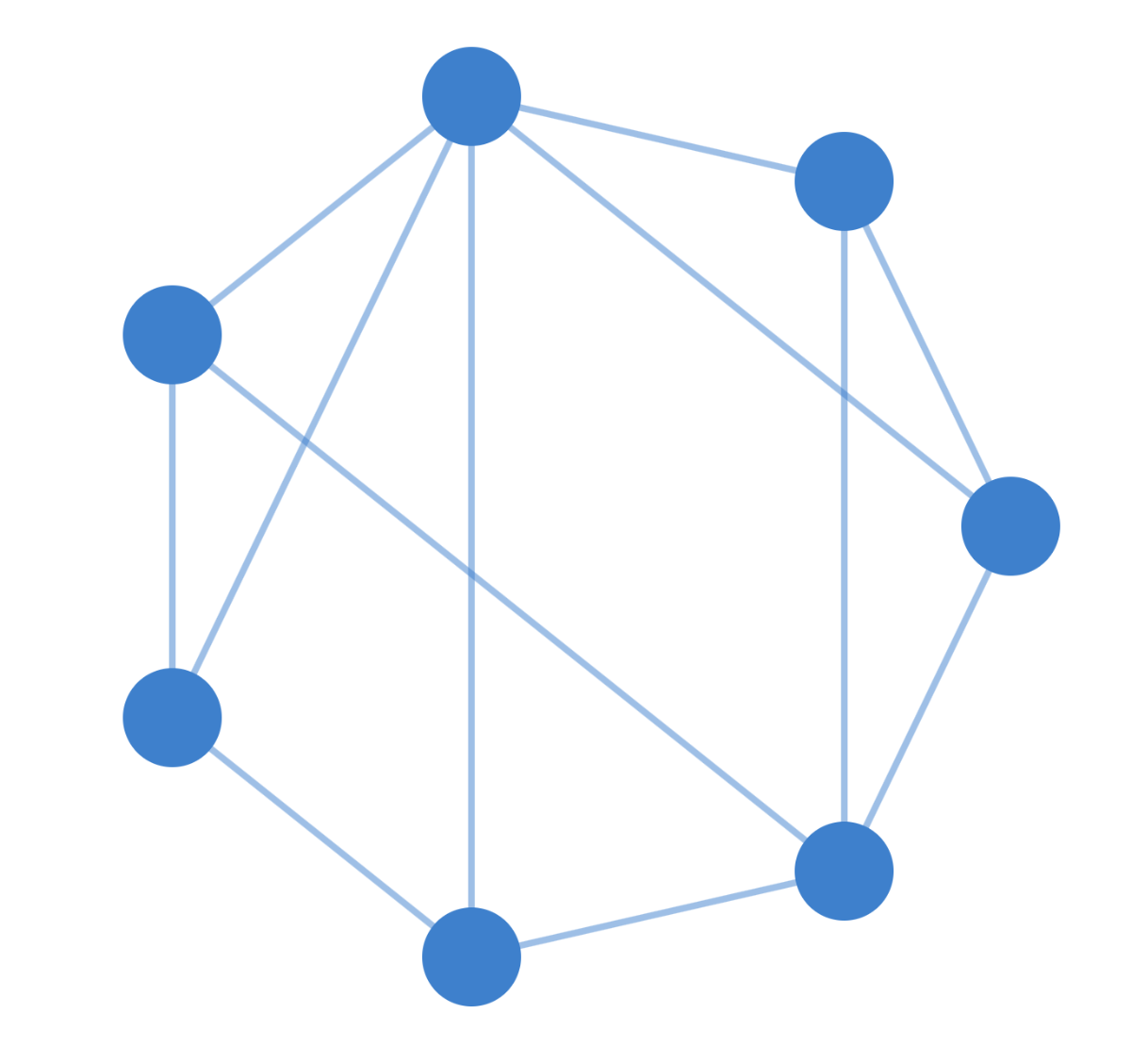
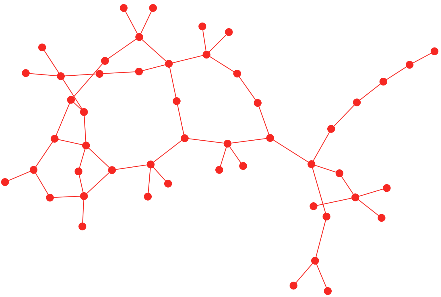
A force-directed layout highlights the underlying topology of the graph. For example, you can visually identify clusters, cliques, and bridges. These sorts of benefits are only apparent if the graph has these properties. If the graph is too highly connected or too unstructured, then a force-directed graph will tend to produce a hairball.

If you get a hairball with one of these layouts, consider selecting a smaller or more specific subgraph to display. Tweaking the forces used in the physics simulation (i.e. by tweaking the options), can also help to give better results. This process of tweaking is typically done by trial and error. Adding sliders to a debug panel in your app can help to find values that are well suited to your data.

fcose, cose-bilkent, & cose : These layouts represent a progression in the sophistication of force-directed layouts. As their names suggest, each of these layouts works well with compound graphs. The cose layout is the first JS implementation of the CoSE algorithm, as specified in its paper. It is integrated into the Cytoscape library itself. It has a fast implementation of CoSE, but it lacks the enhancements of later versions on the algorithm. You may have to tweak the parameters of cose more as compared to other force-directed layouts in order to get a good result. The cose-bilkent layout is a bit more sophisticated than cose. It often gives better results by default, but it can be more expensive to run. The fcose layout is the latest and greatest version of CoSE. It gives the best results of these three layouts, and it is also generally the fastest. If you are considering a force-directed layout, fcose should be the first layout that you try.

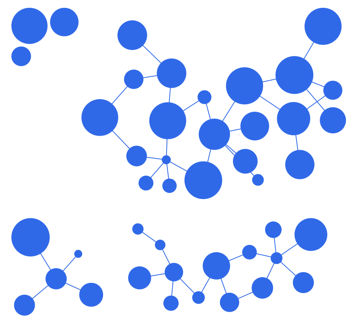
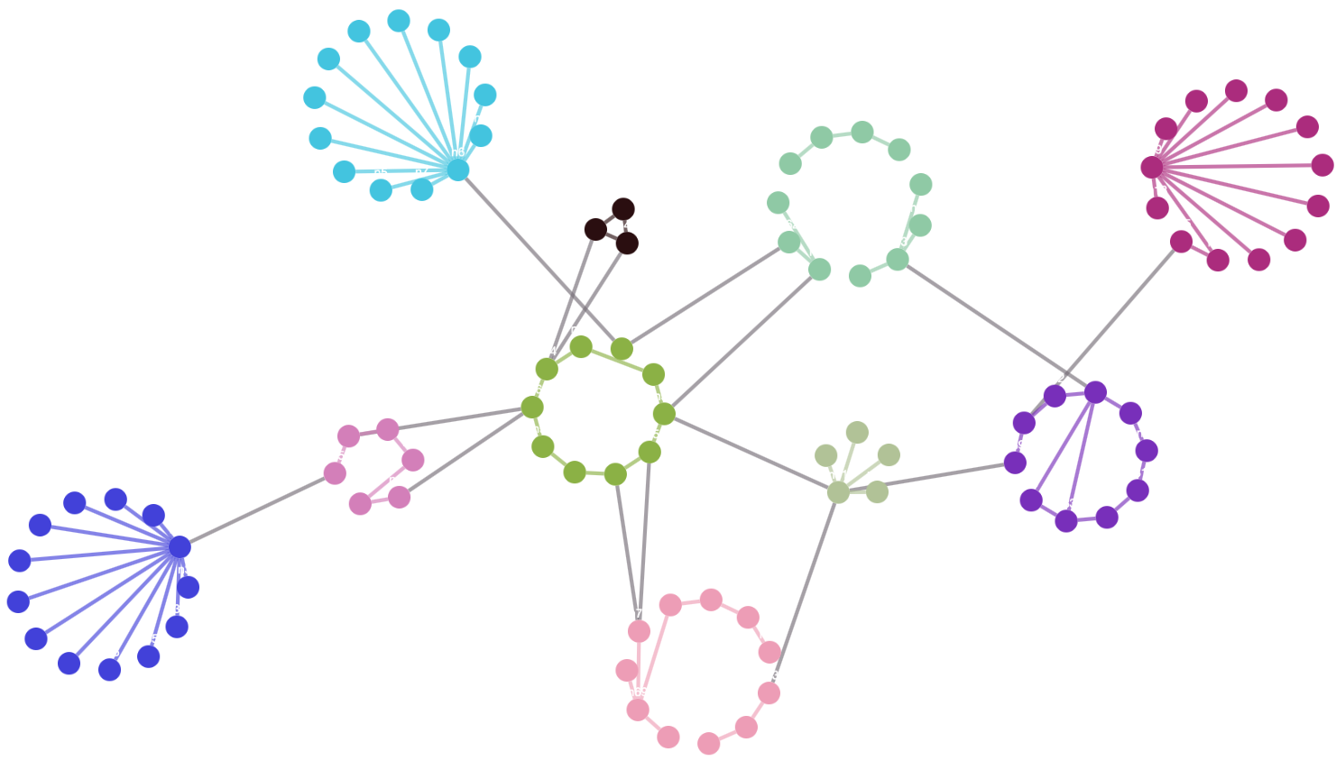
cola : The cola layout differentiates itself by allowing for setting constraints on top of the traditional force-directed physics simulation. If you want to set your own rules for how some nodes are organised, then cola is a good fit. This layout also tends to create smooth transitions in node position from one iteration to the next, so it is well suited to successive or infinite runs of the layout.

cise : The cise layout organises the nodes into clusters. Each cluster is represented as a circle. Similar to the avsdf layout, this layout tries to avoid edge overlap within each circle. The clusters are positioned using a force-directed algorithm. If you have well defined clusters in your graph, the cise layout is a good fit.

elk : The elk layout contains the stress and force algorithms. These algorithms can be combined with the disco algorithm of elk so that the disconnected components of the graph do not overlap, though most other force-directed layouts do component packing without additional configuration. The force algorithm is basic, but the stress algorithm can give aesthetically pleasing results. The use of disco is notable, as it can be used after any non-elk layout — or combination of layouts — to perform component packing. Note that elk includes many different layout algorithms, so its file size is comparatively large.

Advanced layout use cases

Interactive use of layouts

The most obvious use for a layout is to set the initial positions of the nodes in a graph so that the user has something to see. However, there are other situations where layouts can be very useful for interactivity.

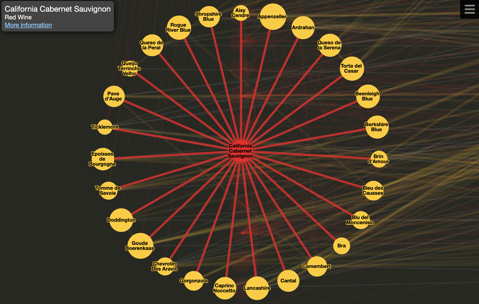
Consider the case where the user is interested in just a particular part of the visible graph. The Wine & Cheese Map is an example of this. Say the user is the hostess of an upcoming party. She has a number of bottles of wine at home, but she isn’t sure what to serve with them. While the default view of the app gives a good sense of the overall landscape of wine-cheese pairings — red wine on the left, cheese in the centre, and white wine on the right — it is difficult to see pairings for a particular wine of interest. The user taps on one of the wines she has at home, and the app uses a layout to help her easily see exactly which cheeses pair well.

Interactivity is key to this example. The user needs to specify which wine or cheese she wants to pair in order to give this highlighted view. Equally important are the details of how the layout is applied.

In this example, a concentric layout is applied only to neighbourhood of the tapped node, while the rest of the graph remains the same. The tapped node remains stationary relative to the overall graph, both in the case of applying the highlight state and in the case of removing the highlight state. This helps the user to maintain her frame of reference.

The use of animation in this layout also helps to maintain the user’s frame of reference. The animated layout provides a smooth transition between the highlighted state and the unhighlighted state. This effect is made even more valuable to the user by always starting a highlight animation from the global frame of reference: The user can click one node after another to explore links in a chain, all the while maintaining both a local and a global frame of reference.

For instance, perhaps the user wants a pairing with California Cabernet Sauvignon. Cantal looks like a good pairing so she taps it out of curiousity. She notes that Lancashire is a similar cheese, and she taps it to explore further. She’s hit the jackpot. Lancashire not only pairs well with California Cabernet Sauvignon but it also pairs well with Syrah, which she also happens to have on hand. This sort of exploration and discovery is only possible because of the use of interactive layout within the app.

Headless use of layouts

A layout is typically run in order to show an organisation of the nodes in a graph at runtime. However, there other instances where it is useful to run a layout within a headless Cytoscape instance.

A common motivation for running a layout headlessly is to generate a preview image. For instance, you may have a number of graphs stored on the server and the user has to choose one of them. In order to clearly and efficiently display this choice on the client, you can generate and cache a thumbnail image for each graph on the server. The Cytosnap library makes image generation easy. Simply specify your elements and layout options in the same JSON format as you would use to initialise Cytoscape. Cytosnap then returns the image.

Another common case for running a layout headlessly is for performance. You may find that a particular layout, or set of layouts, works well for your app. In many cases, you can run the layout directly on the client. In other cases, the layout might be too slow for the sort of user experience you’d like to create. In order to give an instant result to a user, you can precompute and cache the result of the layout on your app’s server.

The simplest approach for precomputed layouts is to run Cytoscape directly in Node. A headless instance does not have style enabled by default, so setting options.styleEnabled: true in your Cytoscape initialisation options can give a better layout result. Node dimensions are the most important aspect of styling for layouts, as this information can be used by some layouts to avoid overlap.

A slightly more involved approach for precomputed layouts is to use Cytosnap. The main purpose for Cytosnap is to generate images, but Cytosnap can alternatively return JSON that contains node positions (resolvesTo: 'json'). Because Cytosnap uses a headless browser instance, it is able to leverage rendered style dimensions (e.g. label dimensions) in addition to stylesheet-specified dimensions. This gives Cytosnap a bit of an edge over using Cytoscape directly at the cost of the overhead of running and starting a headless browser instance.

Batching and layouts

Batching is a good way to minimise the performance impact of style changes, but there are caveats to consider when pairing batching with layouts. If you use batching in your app, take these caveats into consideration when applying layouts.

A layout is dependent on reading style information in order to determine the dimensions of nodes. Those dimensions are important for the layout to make use of overlap avoidance. The dimensions of nodes, as determined by style application, must be available before starting a layout.

Therefore, you should generally ensure that batching has completed prior to running a layout. The pattern would typically look like the following example:

cy.batch(() => {
  // do my style updates here
  cy.nodes().addClass('foo');
  cy.edges().removeClass('bar');
  
  // maybe some more style changes...
});

cy.layout(myLayoutOptions).run();

There is a case to be made for running a layout within a batch cycle, albeit rare. An example would be running two layouts at the same time, with one layout on the first subgraph and the second layout on the second subgraph. In this case, the batching may help to make sure that the two layouts show a result at once — especially on slow devices. It is important to note that a style batch cycle must remain separate from a layout batch cycle. This pattern would look similar to the following code example:

cy.batch(() => {
  // do my style updates here
  cy.nodes().addClass('foo');
  cy.edges().removeClass('bar');
  
  // maybe some more style changes...
});

cy.startBatch();

const getLayoutstop = layout => layout.promiseOn('layoutstop');
const runLayout = layout => layout.run();

const layouts = [
  subgraph1.layout(options1),
  subgraph2.layout(options2)
];

const layoutstops = layouts.map(getLayoutstop);

layouts.forEach(runLayout);

await Promise.all(layoutstops);

cy.endBatch();

If you can guarantee that the size of nodes have not been changed in your style batch cycle, then you may be able to combine style application and layout into a single batch cycle. Note that the nodes must have had style applied at least once for this to hold true. This means that you must not put calls to functions such as cy.add() in a layout batch cycle.

Conclusion

This tutorial should serve as a good starting point to help you decide when and how to use layouts in your apps. For more details on the available layout algorithms, refer to the documentation for the built-in layouts and the documentation for the layout extensions.

Experiment with layouts in your apps. That experimentation can help you unlock a lot of value that your app can provide to your users.